[PythonRobotics 분석] PID편
오늘은 PID, LQR, MPC에 대한 구현을 해놓은 pythonRobotics를 비교해보면서 이론이 실제로 어떻게 적용됬는지 알아보려고 한다.
먼저 너무나도 잘알려져 있는 PID편에 다루겠다.
Rear wheel feedback control
상태에 대한 정의 및 kinematics 모델
class State:
    def __init__(self, x=0.0, y=0.0, yaw=0.0, v=0.0, direction=1):
        self.x = x
        self.y = y
        self.yaw = yaw
        self.v = v
        self.direction = direction

    def update(self, a, delta, dt):
        self.x   = self.x + self.v * math.cos(self.yaw) * dt
        self.y   = self.y + self.v * math.sin(self.yaw) * dt
        self.yaw = self.yaw + self.v / L * math.tan(delta) * dt
self.v = self.v + a * dt- 상태
- \( x, y \): 차량 위치
- \( \theta \): 차량의 (방향)
- \( v \): 속도
- \( L \): 앞바퀴와 뒷바뀌 사이의 거리
- \( \delta \) : 조향각
- kinematics model
$$ \begin{aligned} x_{t+1} &= x_t + v \cos(\theta) \cdot dt \\ y_{t+1} &= y_t + v \sin(\theta) \cdot dt \\ \theta_{t+1} &= \theta_t + \frac{v}{L} \tan(\delta) \cdot dt \\ v_{t+1} &= v + a \cdot dt \end{aligned} $$
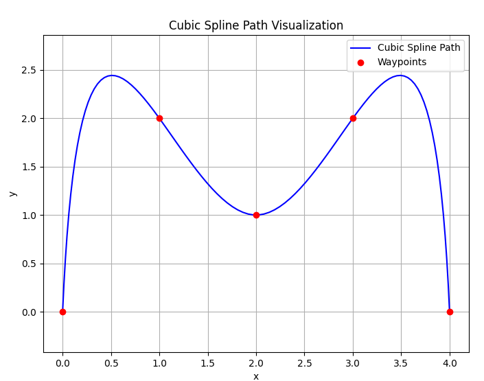
경로 생성
class CubicSplinePath:
    def __init__(self, x, y):
        x, y = map(np.asarray, (x, y))
        s = np.append([0],(np.cumsum(np.diff(x)**2) + np.cumsum(np.diff(y)**2))**0.5)

        self.X = interpolate.CubicSpline(s, x)
        self.Y = interpolate.CubicSpline(s, y)

        self.dX = self.X.derivative(1)
        self.ddX = self.X.derivative(2)

        self.dY = self.Y.derivative(1)
        self.ddY = self.Y.derivative(2)

        self.length = s[-1]
1. 유클리드 거리계산 + 누적 거리 계산
$$ \Delta s_i = \sqrt{\sum_{j=0}^{i-1}(x_{i+1} - x_i)^2 + \sum_{j=0}^{i-1}(y_{i+1} - y_i)^2} $$
2. x와 y의 위치를 거리를 통하여 cubic spline 보간한다. 이를 통해, x,y의 좌표집합은 연속적인 그래프가된다.
경로에서의 오차
    def calc_track_error(self, x, y, s0):
        ret = self.__find_nearest_point(s0, x, y)
        s = ret[0][0]
        e = ret[1]      # 근접 거리 (오차)

        k   = self.calc_curvature(s)   # 곡률
        yaw = self.calc_yaw(s)         # 경로 방향

        dxl = self.X(s) - x
        dyl = self.Y(s) - y
        angle = pi_2_pi(yaw - math.atan2(dyl, dxl))  # 차량에서 경로를 바라보는 방향

        if angle < 0:
            e *= -1

        return e, k, yaw, s
track가 실제 로봇의 오차를 계산한다.
후륜 feedback제어
def rear_wheel_feedback_control(state, e, k, yaw_ref):
    v = state.v
    th_e = pi_2_pi(state.yaw - yaw_ref)

    omega = v * k * math.cos(th_e) / (1.0 - k * e) - \
        KTH * abs(v) * th_e - KE * v * math.sin(th_e) * e / th_e

    if th_e == 0.0 or omega == 0.0:
        return 0.0

    delta = math.atan2(L * omega / v, 1.0)

return delta- 방향 오차 \( \theta_e \)
$$ \theta_e = \theta - \theta_{\text{ref}} $$
- 제어 입력(각속도) \( \omega \)
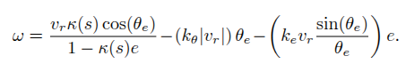
- \( \kappa \): 경로 곡률
- \( e \): 횡방향 오차
- \( v_r \): 뒷 바퀴 속도
- \( \theta_e \): 방향 오차
- \( K_{\theta}, K_e \): 튜닝 파라미터
- 조향각 \( \delta \):
$$ \delta = \tan^{-1}\left( \frac{L \cdot \omega}{v} \right) $$
https://arxiv.org/pdf/1604.07446#page=18.41 해당 논문의 19-20참조
Target Speed와, 방향성 정하기
def calc_target_speed(state, yaw_ref):
    target_speed = 10.0 / 3.6

    dyaw = yaw_ref - state.yaw
    switch = math.pi / 4.0 <= dyaw < math.pi / 2.0

    if switch:
        state.direction *= -1
        return 0.0

    if state.direction != 1:
        return -target_speed

    return target_speed
직진만 하는 것이 아닌 후진도 할수 있는 상태가 된다.
P제어
def pid_control(target, current):
    a = Kp * (target - current)
    return a
사실상 P제어에 가깝다.
오차가 없는 세상에
최종 정리
    while T >= time:
        e, k, yaw_ref, s0 = path_ref.calc_track_error(state.x, state.y, s0)
        di = rear_wheel_feedback_control(state, e, k, yaw_ref)

        speed_ref = calc_target_speed(state, yaw_ref)
        ai = pid_control(speed_ref, state.v)
        state.update(ai, di, dt)

        time = time + dt
경로는 cubic spline 보간 방식을 통해 생성되며, 상당히 곡률이 심하게 변하는 형태일 수 있다.
이떄, 차량이 관성 또는 기존 속도로 인해 곧바로 목표 경로를 추종하기 어려워진다.
경로와 실제 차량 사이에 오차가 발생하게 되고,이를 극복하기 위해 다음과 같은 제어 과정을 수행한다:
- 경로 오차(e), 곡률(k), 목표 방향(yaw_ref)를 계산하여 현재 상태와의 차이를 구함
- 조향각(di)를 재계산하고,
- 속도 제어는 PID 기반의 가속도(ai) 로 조정되며
- 계산된 조향각과 가속도를 기반으로 차량의 상태를 갱신해 나간다.
결과적으로 차량은 반복적으로 오차를 줄이면서 경로를 따라가도록 유도된다.
PID제어로의 수정
Kp = 0.9  # 비례 게인
Ki = 0.1  # 적분 게인
Kd = 0.3  # 미분 게인

def pid_control(target, current):
    global integral_v, prev_v_error
    error = target - current
    integral_v += error * dt
    derivative = (error - prev_v_error) / dt

    a = Kp * error + Ki * integral_v + Kd * derivative
    prev_v_error = error
    return a
PID제어로 수정하고 PID값을 수정해보았다. 기존 P제어에서는 kp 1.0을 사용
PID제어 특성상 튜닝이다~
다음편은 LQR에 대해서 다루겠다
Reference